Notes
Suppose we wish to summarize the following dataset of 18 numbers:
| 38 | 11 | 66 | 9 | 6 | 26 |
| 5 | 38 | 9 | 40 | 20 | 19 |
| 41 | 26 | 12 | 44 | 8 | 52 |
Graphical summaries
- List the data in increasing order: 5, 6, 8, 9, 9, 11, 12, 19, 20, 26, 26, 38, 38, 40, 41, 44, 52, 66.
- A stem-and-leaf plot quickly summarizes numerical data like this without the need for special software. For example:
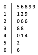
In this case, the stem on the left represents the tens column and each number is represented by one of the unit digits in the leaf on the right. - A histogram groups the data into equal-size intervals and creates a bar graph from the resulting counts:
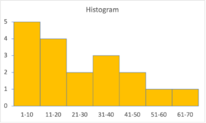
So, there are 5 values between 1 and 10, 4 values between 11 and 20, and so on. - A pie graph also groups the data into intervals, but the intervals need not be equal-size:
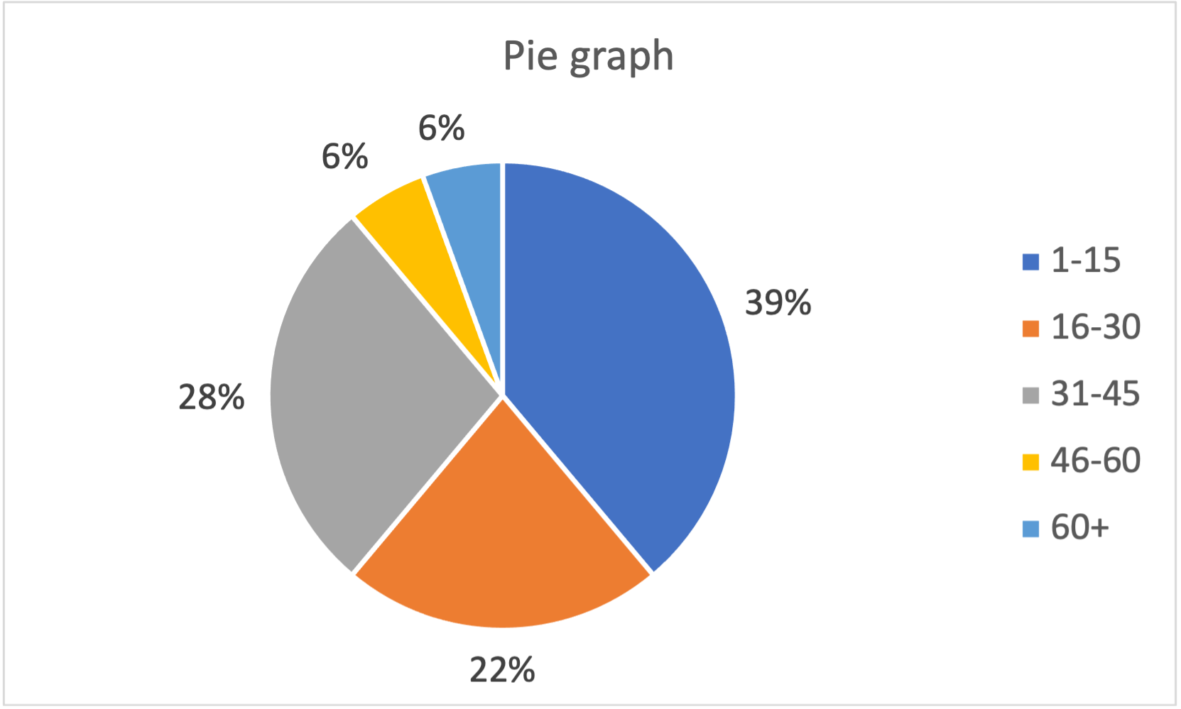
So, 39% of the data are between 1 and 15, 22% are between 16 and 30, and so on. - Together, the graphical summaries tell us about the distribution of the data: the values range between 5 and 66 asymmetrically, with more values nearer the lower end of the range than the upper end. Half the data is 20 or less and a little over 10% is greater than 50.
Numerical summaries
- Two summaries provide alternative measures of the “centre” of the distribution.
- The mean is the total of all the data values divided by the number of data values: (5 + 6 + 8 + … + 52 + 66) / 18 = 470/18 = 26.1.
- The median is the value in the middle of the ordered data (if there is an odd number of data values) or the mean of the two numbers in the middle (if there is an even number of data values). In this case, there are 18 data values, so the median is the mean of the 9th and 10th data values in the ordered list above, i.e., (20 + 26) / 2 = 46/2 = 23.
- The mean is a more meaningful measure of the centre for data with a reasonably symmetric distribution. The median is a more meaningful measure of the centre for data with a strong asymmetric distribution. Here, the distribution is asymmetric, so the median is more meaningful. Since there are a couple of data values much higher than the rest (52 and 66), the mean is “pulled upwards” so that it is greater than the median.
- Quartiles divide the data into quarters. There are different methods to calculate quartiles, but one simple method is the following.
- The first quartile (or lower quartile) is the median of the lower half of the ordered data, i.e., the 5th data value, 9.
- The second quartile is the median, i.e., 23.
- The third quartile (or upper quartile) is the median of the upper half of the ordered data, i.e., the 14th data value, 40.
- Half the data lie between the first and third quartiles and the difference between the first and third quartiles is known as the interquartile range: IQR = 40 – 9 = 31.
The video below works through some examples of summarizing data graphically and numerically.
Video Tips
Practice Exercises
Do the following exercises to practice working with graphical and numerical summaries of data.
